24 Waveguides

24–1The transmission line
In the last chapter we studied what happened to the lumped elements of circuits when they were operated at very high frequencies, and we were led to see that a resonant circuit could be replaced by a cavity with the fields resonating inside. Another interesting technical problem is the connection of one object to another, so that electromagnetic energy can be transmitted between them. In low-frequency circuits the connection is made with wires, but this method doesn’t work very well at high frequencies because the circuits would radiate energy into all the space around them, and it is hard to control where the energy will go. The fields spread out around the wires; the currents and voltages are not “guided” very well by the wires. In this chapter we want to look into the ways that objects can be interconnected at high frequencies. At least, that’s one way of presenting our subject.
Another way is to say that we have been discussing the behavior of waves in free space. Now it is time to see what happens when oscillating fields are confined in one or more dimensions. We will discover the interesting new phenomenon when the fields are confined in only two dimensions and allowed to go free in the third dimension, they propagate in waves. These are “guided waves”—the subject of this chapter.
We begin by working out the general theory of the transmission line. The ordinary power transmission line that runs from tower to tower over the countryside radiates away some of its power, but the power frequencies ($50$–$60$ cycles/sec) are so low that this loss is not serious. The radiation could be stopped by surrounding the line with a metal pipe, but this method would not be practical for power lines because the voltages and currents used would require a very large, expensive, and heavy pipe. So simple “open lines” are used.
For somewhat higher frequencies—say a few kilocycles—radiation can already be serious. However, it can be reduced by using “twisted-pair” transmission lines, as is done for short-run telephone connections. At higher frequencies, however, the radiation soon becomes intolerable, either because of power losses or because the energy appears in other circuits where it isn’t wanted. For frequencies from a few kilocycles to some hundreds of megacycles, electromagnetic signals and power are usually transmitted via coaxial lines consisting of a wire inside a cylindrical “outer conductor” or “shield.” Although the following treatment will apply to a transmission line of two parallel conductors of any shape, we will carry it out referring to a coaxial line.
We take the simplest coaxial line that has a central conductor, which we suppose is a thin hollow cylinder, and an outer conductor which is another thin cylinder on the same axis as the inner conductor, as in Fig. 24–1. We begin by figuring out approximately how the line behaves at relatively low frequencies. We have already described some of the low-frequency behavior when we said earlier that two such conductors had a certain amount of inductance per unit length or a certain capacity per unit length. We can, in fact, describe the low-frequency behavior of any transmission line by giving its inductance per unit length, $L_0$ and its capacity per unit length, $C_0$. Then we can analyze the line as the limiting case of the $L$-$C$ filter as discussed in Section 22–6. We can make a filter which imitates the line by taking small series elements $L_0\,\Delta x$ and small shunt capacities $C_0\,\Delta x$, where $\Delta x$ is an element of length of the line. Using our results for the infinite filter, we see that there would be a propagation of electric signals along the line. Rather than following that approach, however, we would now rather look at the line from the point of view of a differential equation.
Suppose that we see what happens at two neighboring points along the transmission line, say at the distances $x$ and $x+\Delta x$ from the beginning of the line. Let’s call the voltage difference between the two conductors $V(x)$, and the current along the “hot” conductor $I(x)$ (see Fig. 24–2). If the current in the line is varying, the inductance will give us a voltage drop across the small section of line from $x$ to $x+\Delta x$ in the amount \begin{equation*} \Delta V=V(x+\Delta x)-V(x)=-L_0\,\Delta x\,\ddt{I}{t}. \end{equation*} Or, taking the limit as $\Delta x\to0$, we get \begin{equation} \label{Eq:II:24:1} \ddp{V}{x}=-L_0\,\ddp{I}{t}. \end{equation} The changing current gives a gradient of the voltage.
Referring again to the figure, if the voltage at $x$ is changing, there must be some charge supplied to the capacity in that region. If we take the small piece of line between $x$ and $x+\Delta x$, the charge on it is $q=C_0\,\Delta x V$. The time rate-of-change of this charge is $C_0\,\Delta x\,dV/dt$, but the charge changes only if the current $I(x)$ into the element is different from the current $I(x+\Delta x)$ out. Calling the difference $\Delta I$, we have \begin{equation*} \Delta I=-C_0\,\Delta x\,\ddt{V}{t}. \end{equation*} Taking the limit as $\Delta x\to0$, we get \begin{equation} \label{Eq:II:24:2} \ddp{I}{x}=-C_0\,\ddp{V}{t}. \end{equation} So the conservation of charge implies that the gradient of the current is proportional to the time rate-of-change of the voltage.
Equations (24.1) and (24.2) are then the basic equations of a transmission line. If we wish, we could modify them to include the effects of resistance in the conductors or of leakage of charge through the insulation between the conductors, but for our present discussion we will just stay with the simple example.
The two transmission line equations can be combined by differentiating one with respect to $t$ and the other with respect to $x$ and eliminating either $V$ or $I$. Then we have either \begin{equation} \label{Eq:II:24:3} \frac{\partial^2V}{\partial x^2} =C_0L_0\,\frac{\partial^2V}{\partial t^2} \end{equation} or \begin{equation} \label{Eq:II:24:4} \frac{\partial^2I}{\partial x^2} =C_0L_0\,\frac{\partial^2I}{\partial t^2} \end{equation}
Once more we recognize the wave equation in $x$. For a uniform transmission line, the voltage (and current) propagates along the line as a wave. The voltage along the line must be of the form $V(x,t)=f(x-vt)$ or $V(x,t)=g(x+vt)$, or a sum of both. Now what is the velocity $v$? We know that the coefficient of the $\partial^2/\partial t^2$ term is just $1/v^2$, so \begin{equation} \label{Eq:II:24:5} v=\frac{1}{\sqrt{L_0C_0}}. \end{equation}
We will leave it for you to show that the voltage for each wave in a line is proportional to the current of that wave and that the constant of proportionality is just the characteristic impedance $z_0$. Calling $V_+$ and $I_+$ the voltage and current for a wave going in the plus $x$-direction, you should get \begin{equation} \label{Eq:II:24:6} V_+=z_0I_+. \end{equation} Similarly, for the wave going toward minus $x$ the relation is \begin{equation*} V_-=z_0I_-. \end{equation*}
The characteristic impedance—as we found out from our filter equations—is given by \begin{equation} \label{Eq:II:24:7} z_0=\sqrt{\frac{L_0}{C_0}}, \end{equation} and is, therefore, a pure resistance.
To find the propagation speed $v$ and the characteristic impedance $z_0$ of a transmission line, we have to know the inductance and capacity per unit length. We can calculate them easily for a coaxial cable, so we will see how that goes. For the inductance we follow the ideas of Section 17–8, and set $\tfrac{1}{2}LI^2$ equal to the magnetic energy which we get by integrating $\epsO c^2B^2/2$ over the volume. Suppose that the central conductor carries the current $I$; then we know that $B=I/2\pi\epsO c^2r$, where $r$ is the distance from the axis. Taking as a volume element a cylindrical shell of thickness $dr$ and of length $l$, we have for the magnetic energy \begin{equation*} U=\frac{\epsO c^2}{2}\int_a^b\biggl( \frac{I}{2\pi\epsO c^2r} \biggr)^2l\,2\pi r\,dr, \end{equation*} where $a$ and $b$ are the radii of the inner and outer conductors, respectively. Carrying out the integral, we get \begin{equation} \label{Eq:II:24:8} U=\frac{I^2l}{4\pi\epsO c^2}\ln\frac{b}{a}. \end{equation} Setting the energy equal to $\tfrac{1}{2}LI^2$, we find \begin{equation} \label{Eq:II:24:9} L=\frac{l}{2\pi\epsO c^2}\ln\frac{b}{a}. \end{equation} It is, as it should be, proportional to the length $l$ of the line, so the inductance per unit length $L_0$ is \begin{equation} \label{Eq:II:24:10} L_0=\frac{\ln(b/a)}{2\pi\epsO c^2}. \end{equation}
We have worked out the charge on a cylindrical condenser (see Section 12–2). Now, dividing the charge by the potential difference, we get \begin{equation*} C=\frac{2\pi\epsO l}{\ln(b/a)}. \end{equation*} The capacity per unit length $C_0$ is $C/l$. Combining this result with Eq. (24.10), we see that the product $L_0C_0$ is just equal to $1/c^2$, so $v=1/\sqrt{L_0C_0}$ is equal to $c$. The wave travels down the line with the speed of light. We point out that this result depends on our assumptions: (a) that there are no dielectrics or magnetic materials in the space between the conductors, and (b) that the currents are all on the surfaces of the conductors (as they would be for perfect conductors). We will see later that for good conductors at high frequencies, all currents distribute themselves on the surfaces as they would for a perfect conductor, so this assumption is then valid.
Now it is interesting that so long as assumptions (a) and (b) are correct, the product $L_0C_0$ is equal to $1/c^2$ for any parallel pair of conductors—even, say, for a hexagonal inner conductor anywhere inside an elliptical outer conductor. So long as the cross section is constant and the space between has no material, waves are propagated at the velocity of light.
No such general statement can be made about the characteristic impedance. For the coaxial line, it is \begin{equation} \label{Eq:II:24:11} z_0=\frac{\ln(b/a)}{2\pi\epsO c}. \end{equation} The factor $1/\epsO c$ has the dimensions of a resistance and is equal to $120\pi$ ohms. The geometric factor $\ln(b/a)$ depends only logarithmically on the dimensions, so for the coaxial line—and most lines—the characteristic impedance has typical values of from $50$ ohms or so to a few hundred ohms.
24–2The rectangular waveguide
The next thing we want to talk about seems, at first sight, to be a striking phenomenon: if the central conductor is removed from the coaxial line, it can still carry electromagnetic power. In other words, at high enough frequencies a hollow tube will work just as well as one with wires. It is related to the mysterious way in which a resonant circuit of a condenser and inductance gets replaced by nothing but a can at high frequencies.
Although it may seem to be a remarkable thing when one has been thinking in terms of a transmission line as a distributed inductance and capacity, we all know that electromagnetic waves can travel along inside a hollow metal pipe. If the pipe is straight, we can see through it! So certainly electromagnetic waves go through a pipe. But we also know that it is not possible to transmit low-frequency waves (power or telephone) through the inside of a single metal pipe. So it must be that electromagnetic waves will go through if their wavelength is short enough. Therefore we want to discuss the limiting case of the longest wavelength (or the lowest frequency) that can get through a pipe of a given size. Since the pipe is then being used to carry waves, it is called a waveguide.
We will begin with a rectangular pipe, because it is the simplest case to analyze. We will first give a mathematical treatment and come back later to look at the problem in a much more elementary way. The more elementary approach, however, can be applied easily only to a rectangular guide. The basic phenomena are the same for a general guide of arbitrary shape, so the mathematical argument is fundamentally more sound.
Our problem, then, is to find what kind of waves can exist inside a rectangular pipe. Let’s first choose some convenient coordinates; we take the $z$-axis along the length of the pipe, and the $x$- and $y$-axes parallel to the two sides, as shown in Fig. 24–3.
We know that when light waves go down the pipe, they have a transverse electric field; so suppose we look first for solutions in which $\FLPE$ is perpendicular to $z$, say with only a $y$-component, $E_y$. This electric field will have some variation across the guide; in fact, it must go to zero at the sides parallel to the $y$-axis, because the currents and charges in a conductor always adjust themselves so that there is no tangential component of the electric field at the surface of a conductor. So $E_y$ will vary with $x$ in some arch, as shown in Fig. 24–4. Perhaps it is the Bessel function we found for a cavity? No, because the Bessel function has to do with cylindrical geometries. For a rectangular geometry, waves are usually simple harmonic functions, so we should try something like $\sin k_xx$.
Since we want waves that propagate down the guide, we expect the field to alternate between positive and negative values as we go along in $z$, as in Fig. 24–5, and these oscillations will travel along the guide with some velocity $v$. If we have oscillations at some definite frequency $\omega$, we would guess that the wave might vary with $z$ like $\cos\,(\omega t-k_zz)$, or to use the more convenient mathematical form, like $e^{i(\omega t-k_zz)}$. This $z$-dependence represents a wave travelling with the speed $v=\omega/k_z$ (see Chapter 29, Vol. I).
So we might guess that the wave in the guide would have the following mathematical form: \begin{equation} \label{Eq:II:24:12} E_y=E_0e^{i(\omega t-k_zz)}\sin k_xx. \end{equation}
Let’s see whether this guess satisfies the correct field equations. First, the electric field should have no tangential components at the conductors. Our field satisfies this requirement; it is perpendicular to the top and bottom faces and is zero at the two side faces. Well, it is if we choose $k_x$ so that one-half a cycle of $\sin k_xx$ just fits in the width of the guide—that is, if \begin{equation} \label{Eq:II:24:13} k_xa=\pi. \end{equation} There are other possibilities, like $k_xa=2\pi$, $3\pi$, $\dotsc$, or, in general, \begin{equation} \label{Eq:II:24:14} k_xa=n\pi, \end{equation} where $n$ is any integer. These represent various complicated arrangements of the field, but for now let’s take only the simplest one, where $k_x=\pi/a$, where $a$ is the width of the inside of the guide.
Next, the divergence of $\FLPE$ must be zero in the free space inside the guide, since there are no charges there. Our $\FLPE$ has only a $y$-component, and it doesn’t change with $y$, so we do have that $\FLPdiv{\FLPE}=0$.
Finally, our electric field must agree with the rest of Maxwell’s equations in the free space inside the guide. That is the same thing as saying that it must satisfy the wave equation \begin{equation} \label{Eq:II:24:15} \frac{\partial^2E_y}{\partial x^2}+ \frac{\partial^2E_y}{\partial y^2}+ \frac{\partial^2E_y}{\partial z^2}- \frac{1}{c^2}\,\frac{\partial^2E_y}{\partial t^2}=0. \end{equation} We have to see whether our guess, Eq. (24.12), will work. The second derivative of $E_y$ with respect to $x$ is just $-k_x^2E_y$. The second derivative with respect to $y$ is zero, since nothing depends on $y$. The second derivative with respect to $z$ is $-k_z^2E_y$, and the second derivative with respect to $t$ is $-\omega^2E_y$. Equation (24.15) then says that \begin{equation*} k_x^2E_y+k_z^2E_y-\frac{\omega^2}{c^2}\,E_y=0. \end{equation*} Unless $E_y$ is zero everywhere (which is not very interesting), this equation is correct if \begin{equation} \label{Eq:II:24:16} k_x^2+k_z^2-\frac{\omega^2}{c^2}=0. \end{equation} We have already fixed $k_x$, so this equation tells us that there can be waves of the type we have assumed if $k_z$ is related to the frequency $\omega$ so that Eq. (24.16) is satisfied—in other words, if \begin{equation} \label{Eq:II:24:17} k_z=\sqrt{(\omega^2/c^2)-(\pi^2/a^2)}. \end{equation} The waves we have described are propagated in the $z$-direction with this value of $k_z$.
The wave number $k_z$ we get from Eq. (24.17) tells us, for a given frequency $\omega$, the speed with which the nodes of the wave propagate down the guide. The phase velocity is \begin{equation} \label{Eq:II:24:18} v=\frac{\omega}{k_z}. \end{equation}
You will remember that the wavelength $\lambda$ of a travelling wave is given by $\lambda=2\pi v/\omega$, so $k_z$ is also equal to $2\pi/\lambda_g$, where $\lambda_g$ is the wavelength of the oscillations along the $z$-direction—the “guide wavelength.” The wavelength in the guide is different, of course, from the free-space wavelength of electromagnetic waves of the same frequency. If we call the free-space wavelength $\lambda_0$, which is equal to $2\pi c/\omega$, we can write Eq. (24.17) as \begin{equation} \label{Eq:II:24:19} \lambda_g=\frac{\lambda_0}{\sqrt{1-(\lambda_0/2a)^2}}. \end{equation}
Besides the electric fields there are magnetic fields that will travel with the wave, but we will not bother to work out an expression for them right now. Since $c^2\FLPcurl{\FLPB}=\ddpl{\FLPE}{t}$, the lines of $\FLPB$ will circulate around the regions in which $\ddpl{\FLPE}{t}$ is largest, that is, halfway between the maximum and minimum of $\FLPE$. The loops of $\FLPB$ will lie parallel to the $xz$-plane and between the crests and troughs of $\FLPE$, as shown in Fig. 24–6.
24–3The cutoff frequency
In solving Eq. (24.16) for $k_z$, there should really be two roots—one plus and one minus. We should write \begin{equation} \label{Eq:II:24:20} k_z=\pm\sqrt{(\omega^2/c^2)-(\pi^2/a^2)}. \end{equation} The two signs simply mean that there can be waves which propagate with a negative phase velocity (toward $-z$), as well as waves which propagate in the positive direction in the guide. Naturally, it should be possible for waves to go in either direction. Since both types of waves can be present at the same time, there will be the possibility of standing-wave solutions.
Our equation for $k_z$ also tells us that higher frequencies give larger values of $k_z$, and therefore smaller wavelengths, until in the limit of large $\omega$, $k$ becomes equal to $\omega/c$, which is the value we would expect for waves in free space. The light we “see” through a pipe still travels at the speed $c$. But now notice that if we go toward low frequencies, something strange happens. At first the wavelength gets longer and longer, but if $\omega$ gets too small the quantity inside the square root of Eq. (24.20) suddenly becomes negative. This will happen as soon as $\omega$ gets to be less than $\pi c/a$—or when $\lambda_0$ becomes greater than $2a$. In other words, when the frequency gets smaller than a certain critical frequency $\omega_c=\pi c/a$, the wave number $k_z$ (and also $\lambda_g$) becomes imaginary and we haven’t got a solution any more. Or do we? Who said that $k_z$ has to be real? What if it does come out imaginary? Our field equations are still satisfied. Perhaps an imaginary $k_z$ also represents a wave.
Suppose $\omega$ is less than $\omega_c$; then we can write \begin{equation} \label{Eq:II:24:21} k_z=\pm ik', \end{equation} where $k'$ is a positive real number: \begin{equation} \label{Eq:II:24:22} k'=\sqrt{(\pi^2/a^2)-(\omega^2/c^2)}. \end{equation} If we now go back to our expression, Eq. (24.12), for $E_y$, we have \begin{equation} \label{Eq:II:24:23} E_y =E_0e^{i(\omega t\mp ik'z)}\sin k_xx, \end{equation} which we can write as \begin{equation} \label{Eq:II:24:24} E_y =E_0e^{\pm k'z}e^{i\omega t}\sin k_xx. \end{equation}
This expression gives an $\FLPE$-field that oscillates with time as $e^{i\omega t}$ but which varies with $z$ as $e^{\pm k'z}$. It decreases or increases with $z$ smoothly as a real exponential. In our derivation we didn’t worry about the sources that started the waves, but there must, of course, be a source someplace in the guide. The sign that goes with $k'$ must be the one that makes the field decrease with increasing distance from the source of the waves.
So for frequencies below $\omega_c=\pi c/a$, waves do not propagate down the guide; the oscillating fields penetrate into the guide only a distance of the order of $1/k'$. For this reason, the frequency $\omega_c$ is called the “cutoff frequency” of the guide. Looking at Eq. (24.22), we see that for frequencies just a little below $\omega_c$, the number $k'$ is small and the fields can penetrate a long distance into the guide. But if $\omega$ is much less than $\omega_c$, the exponential coefficient $k'$ is equal to $\pi/a$ and the field dies off extremely rapidly, as shown in Fig. 24–7. The field decreases by $1/e$ in the distance $a/\pi$, or in only about one-third of the guide width. The fields penetrate very little distance from the source.
We want to emphasize an interesting feature of our analysis of the guided waves—the appearance of the imaginary wave number $k_z$. Normally, if we solve an equation in physics and get an imaginary number, it doesn’t mean anything physical. For waves, however, an imaginary wave number does mean something. The wave equation is still satisfied; it only means that the solution gives exponentially decreasing fields instead of propagating waves. So in any wave problem where $k$ becomes imaginary for some frequency, it means that the form of the wave changes—the sine wave changes into an exponential.
24–4The speed of the guided waves
The wave velocity we have used above is the phase velocity, which is the speed of a node of the wave; it is a function of frequency. If we combine Eqs. (24.17) and (24.18), we can write \begin{equation} \label{Eq:II:24:25} v_{\text{phase}}=\frac{c}{\sqrt{1-(\omega_c/\omega)^2}}. \end{equation} For frequencies above cutoff—where travelling waves exist—$\omega_c/\omega$ is less than one, and $v_{\text{phase}}$ is real and greater than the speed of light. We have already seen in Chapter 48 of Vol. I that phase velocities greater than light are possible, because it is just the nodes of the wave which are moving and not energy or information. In order to know how fast signals will travel, we have to calculate the speed of pulses or modulations made by the interference of a wave of one frequency with one or more waves of slightly different frequencies (see Chapter 48, Vol. I). We have called the speed of the envelope of such a group of waves the group velocity; it is not $\omega/k$ but $d\omega/dk$: \begin{equation} \label{Eq:II:24:26} v_{\text{group}}=\ddt{\omega}{k}. \end{equation} Taking the derivative of Eq. (24.17) with respect to $\omega$ and inverting to get $d\omega/dk$, we find that \begin{equation} \label{Eq:II:24:27} v_{\text{group}}=c\sqrt{1-(\omega_c/\omega)^2}, \end{equation} which is less than the speed of light.
The geometric mean of $v_{\text{phase}}$ and $v_{\text{group}}$ is just $c$, the speed of light: \begin{equation} \label{Eq:II:24:28} v_{\text{phase}}v_{\text{group}}=c^2. \end{equation} This is curious, because we have seen a similar relation in quantum mechanics. For a particle with any velocity—even relativistic—the momentum $p$ and energy $U$ are related by \begin{equation} \label{Eq:II:24:29} U^2=p^2c^2+m^2c^4. \end{equation} But in quantum mechanics the energy is $\hbar\omega$, and the momentum is $\hbar/\lambdabar$, which is equal to $\hbar k$; so Eq. (24.29) can be written \begin{equation} \label{Eq:II:24:30} \frac{\omega^2}{c^2}=k^2+\frac{m^2c^2}{\hbar^2}, \end{equation} or \begin{equation} \label{Eq:II:24:31} k=\sqrt{(\omega^2/c^2)-(m^2c^2/\hbar^2)}, \end{equation} which looks very much like Eq. (24.17) … Interesting!
The group velocity of the waves is also the speed at which energy is transported along the guide. If we want to find the energy flow down the guide, we can get it from the energy density times the group velocity. If the root mean square electric field is $E_0$, then the average density of electric energy is $\epsO E_0^2/2$. There is also some energy associated with the magnetic field. We will not prove it here, but in any cavity or guide the magnetic and electric energies are equal, so the total electromagnetic energy density is $\epsO E_0^2$. The power $dU/dt$ transmitted by the guide is then \begin{equation} \label{Eq:II:24:32} \ddt{U}{t}=\epsO E_0^2abv_{\text{group}}. \end{equation} (We will see later another, more general way of getting the energy flow.)
24–5Observing guided waves
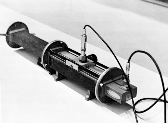
Energy can be coupled into a waveguide by some kind of an “antenna.” For example, a little vertical wire or “stub” will do. The presence of the guided waves can be observed by picking up some of the electromagnetic energy with a little receiving “antenna,” which again can be a little stub of wire or a small loop. In Fig. 24–8, we show a guide with some cutaways to show a driving stub and a pickup “probe”. The driving stub can be connected to a signal generator via a coaxial cable, and the pickup probe can be connected by a similar cable to a detector. It is usually convenient to insert the pickup probe via a long thin slot in the guide, as shown in Fig. 24–8. Then the probe can be moved back and forth along the guide to sample the fields at various positions.
If the signal generator is set at some frequency $\omega$ greater than the cutoff frequency $\omega_c$, there will be waves propagated down the guide from the driving stub. These will be the only waves present if the guide is infinitely long, which can effectively be arranged by terminating the guide with a carefully designed absorber in such a way that there are no reflections from the far end. Then, since the detector measures the time average of the fields near the probe, it will pick up a signal which is independent of the position along the guide; its output will be proportional to the power being transmitted.
If now the far end of the guide is finished off in some way that produces a reflected wave—as an extreme example, if we closed it off with a metal plate—there will be a reflected wave in addition to the original forward wave. These two waves will interfere and produce a standing wave in the guide similar to the standing waves on a string which we discussed in Chapter 49 of Vol. I. Then, as the pickup probe is moved along the line, the detector reading will rise and fall periodically, showing a maximum in the fields at each loop of the standing wave and a minimum at each node. The distance between two successive nodes (or loops) is just $\lambda_g/2$. This gives a convenient way of measuring the guide wavelength. If the frequency is now moved closer to $\omega_c$, the distances between nodes increase, showing that the guide wavelength increases as predicted by Eq. (24.19).
Suppose now the signal generator is set at a frequency just a little below $\omega_c$. Then the detector output will decrease gradually as the pickup probe is moved down the guide. If the frequency is set somewhat lower, the field strength will fall rapidly, following the curve of Fig. 24–7, and showing that waves are not propagated.
24–6Waveguide plumbing
An important practical use of waveguides is for the transmission of high-frequency power, as, for example, in coupling the high-frequency oscillator or output amplifier of a radar set to an antenna. In fact, the antenna itself usually consists of a parabolic reflector fed at its focus by a waveguide flared out at the end to make a “horn” that radiates the waves coming along the guide. Although high frequencies can be transmitted along a coaxial cable, a waveguide is better for transmitting large amounts of power. First, the maximum power that can be transmitted along a line is limited by the breakdown of the insulation (solid or gas) between the conductors. For a given amount of power, the field strengths in a guide are usually less than they are in a coaxial cable, so higher powers can be transmitted before breakdown occurs. Second, the power losses in the coaxial cable are usually greater than in a waveguide. In a coaxial cable there must be insulating material to support the central conductor, and there is an energy loss in this material—particularly at high frequencies. Also, the current densities on the central conductor are quite high, and since the losses go as the square of the current density, the lower currents that appear on the walls of the guide result in lower energy losses. To keep these losses to a minimum, the inner surfaces of the guide are often plated with a material of high conductivity, such as silver.
The problem of connecting a “circuit” with waveguides is quite different from the corresponding circuit problem at low frequencies, and is usually called microwave “plumbing.” Many special devices have been developed for the purpose. For instance, two sections of waveguide are usually connected together by means of flanges, as can be seen in Fig. 24–9. Such connections can, however, cause serious energy losses, because the surface currents must flow across the joint, which may have a relatively high resistance. One way to avoid such losses is to make the flanges as shown in the cross section drawn in Fig. 24–10. A small space is left between the adjacent sections of the guide, and a groove is cut in the face of one of the flanges to make a small cavity of the type shown in Fig. 23–16(c). The dimensions are chosen so that this cavity is resonant at the frequency being used. This resonant cavity presents a high “impedance” to the currents, so relatively little current flows across the metallic joints (at $a$ in Fig. 24–10). The high guide currents simply charge and discharge the “capacity” of the gap (at $b$ in the figure), where there is little dissipation of energy.
Suppose you want to stop a waveguide in a way that won’t result in reflected waves. Then you must put something at the end that imitates an infinite length of guide. You need a “termination” which acts for the guide like the characteristic impedance does for a transmission line—something that absorbs the arriving waves without making reflections. Then the guide will act as though it went on forever. Such terminations are made by putting inside the guide some wedges of resistance material carefully designed to absorb the wave energy while generating almost no reflected waves.
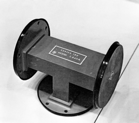
If you want to connect three things together—for instance, one source to two different antennas—then you can use a “T” like the one shown in Fig. 24–11. Power fed in at the center section of the “T” will be split and go out the two side arms (and there may also be some reflected waves). You can see qualitatively from the sketches in Fig. 24–12 that the fields would spread out when they get to the end of the input section and make electric fields that will start waves going out the two arms. Depending on whether electric fields in the guide are parallel or perpendicular to the “top” of the “T,” the fields at the junction would be roughly as shown in (a) or (b) of Fig. 24–12.
Finally, we would like to describe a device called a “unidirectional coupler,” which is very useful for telling what is going on after you have connected a complicated arrangement of waveguides. Suppose you want to know which way the waves are going in a particular section of guide—you might be wondering, for instance, whether or not there is a strong reflected wave. The unidirectional coupler takes out a small fraction of the power of a guide if there is a wave going one way, but none if the wave is going the other way. By connecting the output of the coupler to a detector, you can measure the “one-way” power in the guide.
Figure 24–13 is a drawing of a unidirectional coupler; a piece of waveguide $AB$ has another piece of waveguide $CD$ soldered to it along one face. The guide $CD$ is curved away so that there is room for the connecting flanges. Before the guides are soldered together, two (or more) holes have been drilled in each guide (matching each other) so that some of the fields in the main guide $AB$ can be coupled into the secondary guide $CD$. Each of the holes acts like a little antenna that produces a wave in the secondary guide. If there were only one hole, waves would be sent in both directions and would be the same no matter which way the wave was going in the primary guide. But when there are two holes with a separation space equal to one-quarter of the guide wavelength, they will make two sources $90^\circ$ out of phase. Do you remember that we considered in Chapter 29 of Vol. I the interference of the waves from two antennas spaced $\lambda/4$ apart and excited $90^\circ$ out of phase in time? We found that the waves subtract in one direction and add in the opposite direction. The same thing will happen here. The wave produced in the guide $CD$ will be going in the same direction as the wave in $AB$.
If the wave in the primary guide is travelling from $A$ toward $B$, there will be a wave at the output $D$ of the secondary guide. If the wave in the primary guide goes from $B$ toward $A$, there will be a wave going toward the end $C$ of the secondary guide. This end is equipped with a termination, so that this wave is absorbed and there is no wave at the output of the coupler.
24–7Waveguide modes
The wave we have chosen to analyze is a special solution of the field equations. There are many more. Each solution is called a waveguide “mode.” For example, our $x$-dependence of the field was just one-half a cycle of a sine wave. There is an equally good solution with a full cycle; then the variation of $E_y$ with $x$ is as shown in Fig. 24–14. The $k_x$ for such a mode is twice as large, so the cutoff frequency is much higher. Also, in the wave we studied $\FLPE$ has only a $y$-component, but there are other modes with more complicated electric fields. If the electric field has components only in $x$ and $y$—so that the total electric field is always at right angles to the $z$-direction—the mode is called a “transverse electric” (or TE) mode. The magnetic field of such modes will always have a $z$-component. It turns out that if $\FLPE$ has a component in the $z$-direction (along the direction of propagation), then the magnetic field will always have only transverse components. So such fields are called transverse magnetic (TM) modes. For a rectangular guide, all the other modes have a higher cutoff frequency than the simple TE mode we have described. It is, therefore, possible—and usual—to use a guide with a frequency just above the cutoff for this lowest mode but below the cutoff frequency for all the others, so that just the one mode is propagated. Otherwise, the behavior gets complicated and difficult to control.
24–8Another way of looking at the guided waves
We want now to show you another way of understanding why a waveguide attenuates the fields rapidly for frequencies below the cutoff frequency $\omega_c$. Then you will have a more “physical” idea of why the behavior changes so drastically between low and high frequencies. We can do this for the rectangular guide by analyzing the fields in terms of reflections—or images—in the walls of the guide. The approach only works for rectangular guides, however; that’s why we started with the more mathematical analysis which works, in principle, for guides of any shape.
For the mode we have described, the vertical dimension (in $y$) had no effect, so we can ignore the top and bottom of the guide and imagine that the guide is extended indefinitely in the vertical direction. We imagine then that the guide just consists of two vertical plates with the separation $a$.
Let’s say that the source of the fields is a vertical wire placed in the middle of the guide, with the wire carrying a current that oscillates at the frequency $\omega$. In the absence of the guide walls such a wire would radiate cylindrical waves.
Now we consider that the guide walls are perfect conductors. Then, just as in electrostatics, the conditions at the surface will be correct if we add to the field of the wire the field of one or more suitable image wires. The image idea works just as well for electrodynamics as it does for electrostatics, provided, of course, that we also include the retardations. We know that is true because we have often seen a mirror producing an image of a light source. And a mirror is just a “perfect” conductor for electromagnetic waves with optical frequencies.
Now let’s take a horizontal cross section, as shown in Fig. 24–15, where $W_1$ and $W_2$ are the two guide walls and $S_0$ is the source wire. We call the direction of the current in the wire positive. Now if there were only one wall, say $W_1$, we could remove it if we placed an image source (with opposite polarity) at the position marked $S_1$. But with both walls in place there will also be an image of $S_0$ in the wall $W_2$, which we show as the image $S_2$. This source, too, will have an image in $W_1$, which we call $S_3$. Now both $S_1$ and $S_3$ will have images in $W_2$ at the positions marked $S_4$ and $S_6$, and so on. For our two plane conductors with the source halfway between, the fields are the same as those produced by an infinite line of sources, all separated by the distance $a$. (It is, in fact just what you would see if you looked at a wire placed halfway between two parallel mirrors.) For the fields to be zero at the walls, the polarity of the currents in the images must alternate from one image to the next. In other words, they oscillate $180^\circ$ out of phase. The waveguide field is, then, just the superposition of the fields of such an infinite set of line sources.
We know that if we are close to the sources, the field is very much like the static fields. We considered in Section 7–5 the static field of a grid of line sources and found that it is like the field of a charged plate except for terms that decrease exponentially with the distance from the grid. Here the average source strength is zero, because the sign alternates from one source to the next. Any fields which exist should fall off exponentially with distance. Close to the source, we see the field mainly of the nearest source; at large distances, many sources contribute and their average effect is zero. So now we see why the waveguide below cutoff frequency gives an exponentially decreasing field. At low frequencies, in particular, the static approximation is good, and it predicts a rapid attenuation of the fields with distance.
Now we are faced with the opposite question: Why are waves propagated at all? That is the mysterious part! The reason is that at high frequencies the retardation of the fields can introduce additional changes in phase which can cause the fields of the out-of-phase sources to add instead of cancelling. In fact, in Chapter 29 of Vol. I we have already studied, just for this problem, the fields generated by an array of antennas or by an optical grating. There we found that when several radio antennas are suitably arranged, they can give an interference pattern that has a strong signal in some direction but no signal in another.
Suppose we go back to Fig. 24–15 and look at the fields which arrive at a large distance from the array of image sources. The fields will be strong only in certain directions which depend on the frequency—only in those directions for which the fields from all the sources add in phase. At a reasonable distance from the sources the field propagates in these special directions as plane waves. We have sketched such a wave in Fig. 24–16, where the solid lines represent the wave crests and the dashed lines represent the troughs. The wave direction will be the one for which the difference in the retardation for two neighboring sources to the crest of a wave corresponds to one-half a period of oscillation. In other words, the difference between $r_2$ and $r_0$ in the figure is one-half of the free-space wavelength: \begin{equation} r_2-r_0=\frac{\lambda_0}{2}.\notag \end{equation} The angle $\theta$ is then given by \begin{equation} \label{Eq:II:24:33} \sin\theta=\frac{\lambda_0}{2a}. \end{equation}
There is, of course, another set of waves travelling downward at the symmetric angle with respect to the array of sources. The complete waveguide field (not too close to the source) is the superposition of these two sets of waves, as shown in Fig. 24–17. The actual fields are really like this, of course, only between the two walls of the waveguide.
At points like $A$ and $C$, the crests of the two wave patterns coincide, and the field will have a maximum; at points like $B$, both waves have their peak negative value, and the field has its minimum (largest negative) value. As time goes on the field in the guide appears to be travelling along the guide with a wavelength $\lambda_g$, which is the distance from $A$ to $C$. That distance is related to $\theta$ by \begin{equation} \label{Eq:II:24:34} \cos\theta=\frac{\lambda_0}{\lambda_g}. \end{equation} Using Eq. (24.33) for $\theta$, we get that \begin{equation} \label{Eq:II:24:35} \lambda_g=\frac{\lambda_0}{\cos\theta}= \frac{\lambda_0}{\sqrt{1-(\lambda_0/2a)^2}}, \end{equation} which is just what we found in Eq. (24.19).
Now we see why there is only wave propagation above the cutoff frequency $\omega_0$. If the free-space wavelength is longer than $2a$, there is no angle where the waves shown in Fig. 24–16 can appear. The necessary constructive interference appears suddenly when $\lambda_0$ drops below $2a$, or when $\omega$ goes above $\omega_0=\pi c/a$.
If the frequency is high enough, there can be two or more possible directions in which the waves will appear. For our case, this will happen if $\lambda_0<\tfrac{2}{3}a$. In general, however, it could also happen when $\lambda_0<a$. These additional waves correspond to the higher guide modes we have mentioned.
It has also been made evident by our analysis why the phase velocity of the guided waves is greater than $c$ and why this velocity depends on $\omega$. As $\omega$ is changed, the angle of the free waves of Fig. 24–16 changes, and therefore so does the velocity along the guide.
Although we have described the guided wave as the superposition of the fields of an infinite array of line sources, you can see that we would arrive at the same result if we imagined two sets of free-space waves being continually reflected back and forth between two perfect mirrors—remembering that a reflection means a reversal of phase. These sets of reflecting waves would all cancel each other unless they were going at just the angle $\theta$ given in Eq. (24.33). There are many ways of looking at the same thing.